Local features:

• Detection: Identify the interest points
• Description: Extract feature vector descriptor surrounding each interest point.
• Matching: Determine correspondence between descriptors in two views

Interest Point:

• Expressive texture: The point at which the direction of the boundary of object changes abruptly Intersection point between two or more edge segments

Desired Properties of interest point detectors

• Detect all (or most) true interest points
• No false interest points
• Well localized
• Robust with respect to noise
• Should be fast in detection

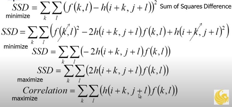
Correlation vs SSD

SSD stands for sum of square differences. Like correlation (to know more about it read my previous blogs ), SSD is a method for seeing the similarity. It is the sum of the squares of the element-wise differences. If you see carefully then in a way correlation and SSD are very similar

Aperture problem

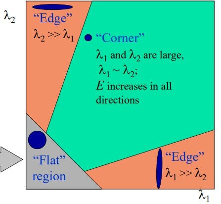
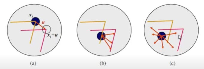The interest points are more like corners because otherwise they will be ambiguous and hence of no use. You can understand this from the diagram above in which we have flat regions (where intensities don’t change much and we have edges, corner is intersection of two of more than two edges). Due to the aperture size (the size of the window ie the size of the filter which we will see later) limits the information so any interest point on the edge as we can see in picture b can have many correspondences (same in the case of the flat regions picture c)

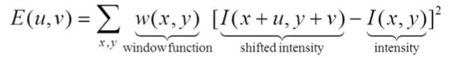
Harris Detector

In a particular window size within the image, we want to detect harris corners (interest points). So we will be taking SSD and apply some window function (probably nature loves gaussian spread :) where u and v are the shifts within the neighbourhood.

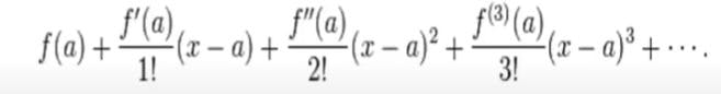
Taylor series
f(x) can be represented at point a in term of its derivatives as

Eigen vectors and Eigen values
The eigen vector x of a matrix A is special vector, with the property Ax = Lambda x where Lambda is eigen value. Finding eigen values of a matrix A: find the roots of det(A- lambda I) = 0 where det is the determinant and I is the identity matrix

As gradient gives a better idea of the texture in the image (pixel values might change a lot due to noise, illumination, angle etc) whereas the gradient will be almost similar of the intensities present. So we will be approximating the I(x+u, y+v) using the Taylor series which I have mentioned briefly above. Then upon simplifying we get

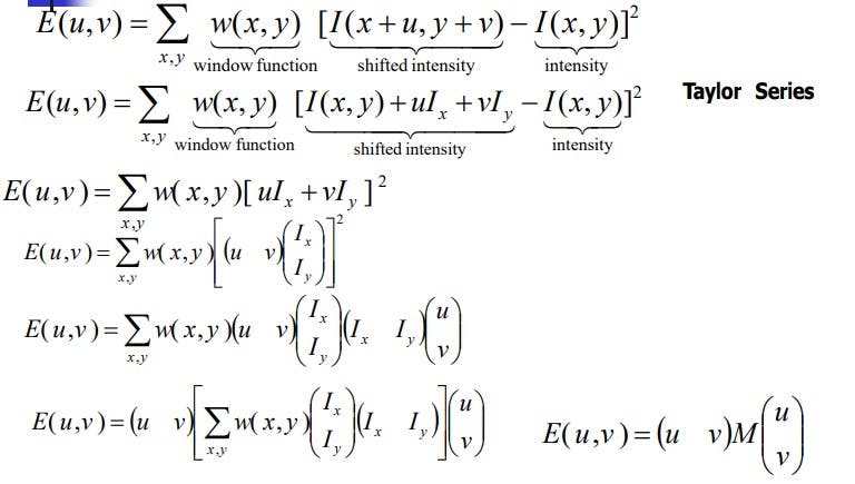
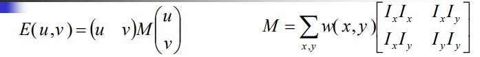
E(u,v) is an equation of an ellipse, where M is the covariance. If lambda1 and lambda2 are eigen values of M then

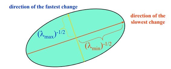
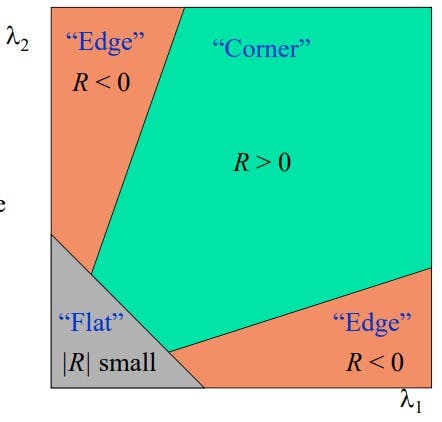
Classification of image points using eigen values of M:

Another way is to calculate R which is det M - k((traceM)^2) and then:

Some other versions of harris detectors are:

• R = lambda1 - alambda2 (triggs)
• R = det(M)/trace(M) = lambda1*lambda2/(lambda1 + lambda2) (szeliski)
• R = lambda1 (shi-tomasi)

This is all about interest points. In the upcoming blogs I will be writing about image-pyramids, SIFT, optical flow etc.

slides taken from mubarak shah’s lectures